Ultra-long Time Series Forecasting

Feng Li

Guanghua School of Management

Peking University

feng.li@gsm.pku.edu.cn

Course home page: https://feng.li/bdcf

Motivation

• Ultra-long time series are increasingly accumulated in many cases.

  • hourly electricity demands
  • daily maximum temperatures
  • streaming data generated in real-time

• Forecasting such long time series is challenging with traditional approaches.

  • time-consuming training process
  • hardware requirements
  • unrealistic assumption about the data generating process

• Some attempts are made in the vast literature.

  • discard the earliest observations
  • allow the model itself to evolve over time
  • apply a model-free prediction

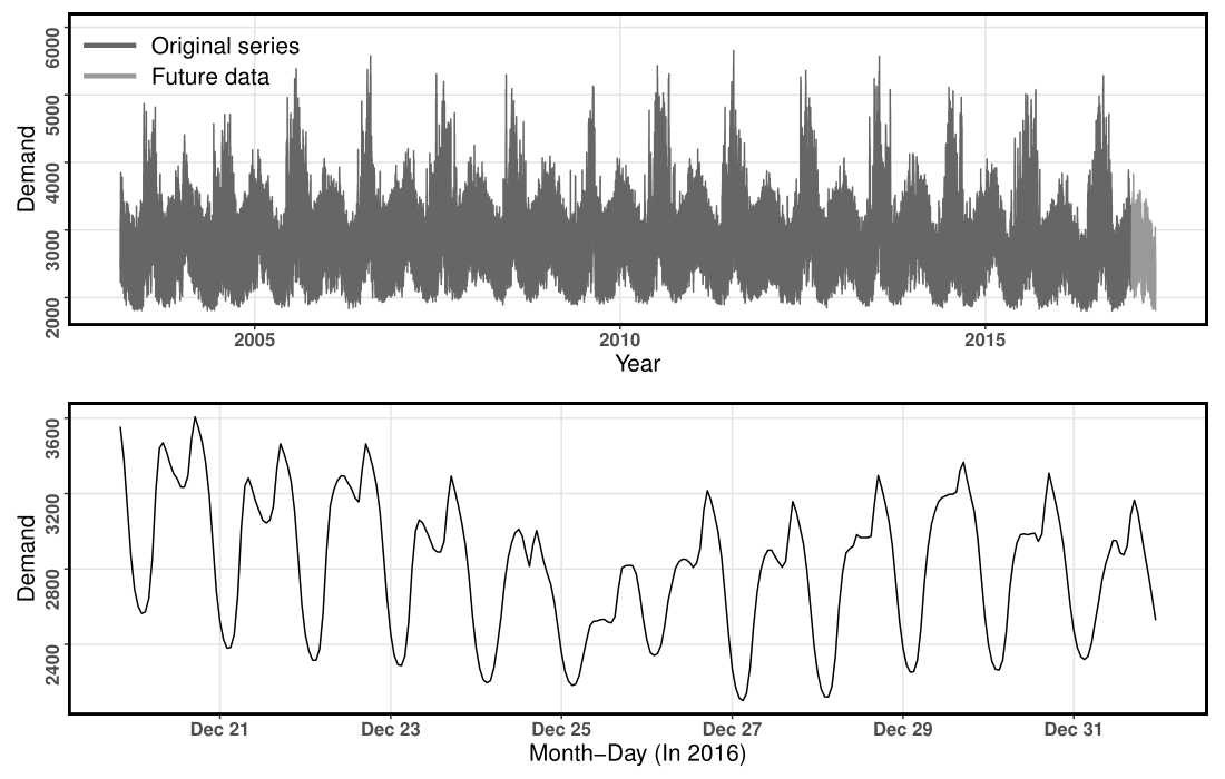
The Global Energy Forecasting Competition 2017 (GEFCom2017)

• Ranging from March 1, 2003 to April 30, 2017 ( $124,171$ time points)

• $10$ hourly electricity load series

• Training periods
  March 1, 2003 - December 31, 2016

• Test periods
  January 1, 2017 - April 30, 2017
  ( $h=2,879$ )

An example series from the GEFCom2017 dataset

Goal of electricity load forecasting

Statistical modeling on distributed systems

• Divide-and-conquer strategy

• Distributed Least Squares Approximation (DLSA, Zhu, Li & Wang, 2021)

  • Solve a large family of regression problems on distributed systems

  • Compute local estimators in worker nodes in a parallel manner

  • Deliver local estimators to the master node to approximate global estimators by taking a weighted average

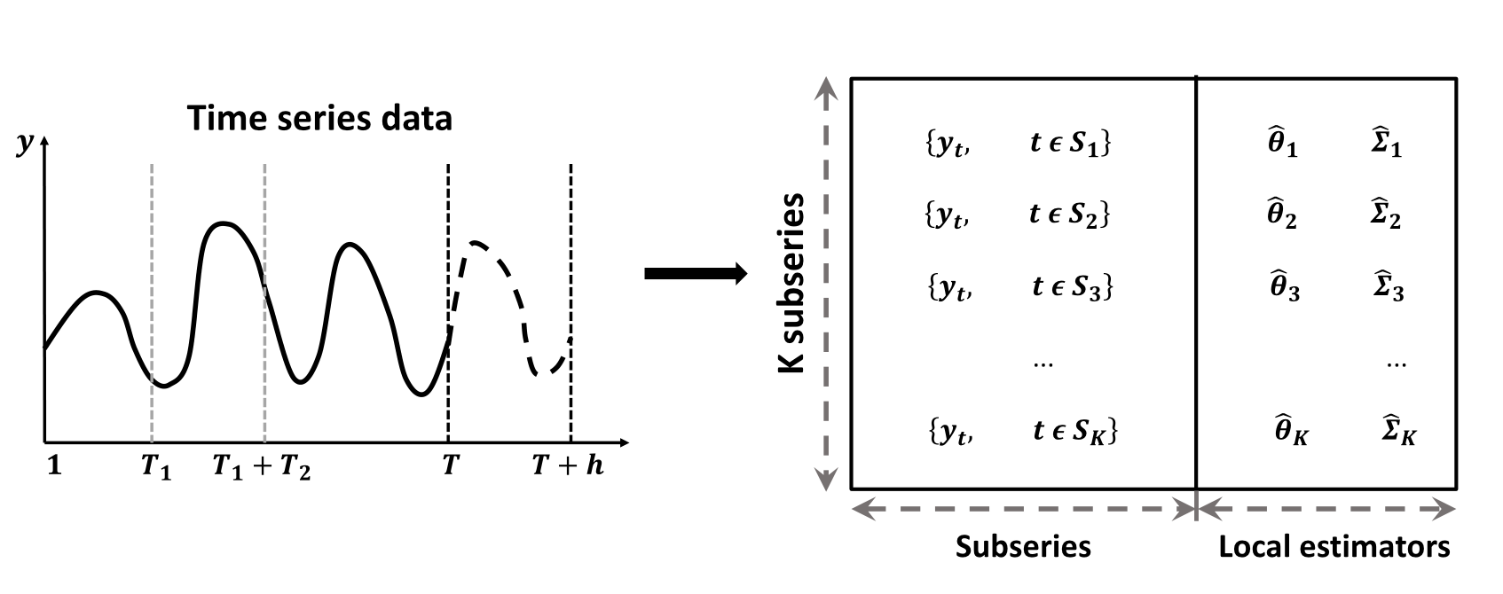
Parameter estimation problem

• For an ultra-long time series $\left\{y_{t}; t=1, 2, \ldots , T \right\}$. Define $\mathcal{S}=\{1, 2, \cdots, T\}$ to be the timestamp sequence.

• The parameter estimation problem can be formulated as $$ f\left( \theta ,\Sigma | y_t, t \in \mathcal{S} \right). $$

• Suppose the whole time series is split into $K$ subseries with contiguous time intervals, that is $\mathcal{S}=\cup_{k=1}^{K} \mathcal{S}_{k}$.

• The parameter estimation problem is transformed into $K$ sub-problems and one combination problem as follows: $$ f\left( \theta ,\Sigma | y_t, t \in \mathcal{S} \right) = g\big( f_1\left( \theta_1 ,\Sigma_1 | y_t, t \in \mathcal{S}_1 \right), \ldots, f_K\left( \theta_K ,\Sigma_K | y_t, t \in \mathcal{S}_K \right) \big). $$

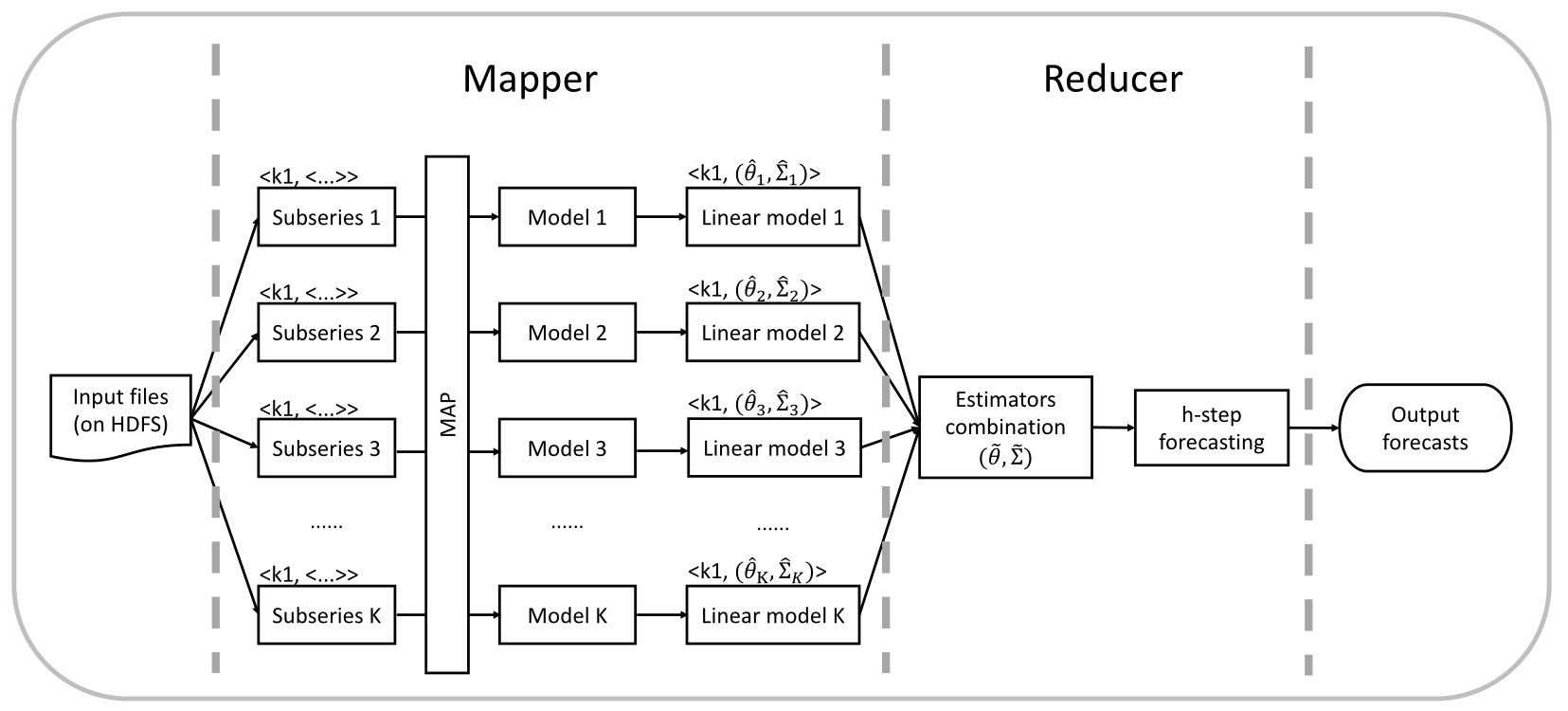
Distributed forecasting

The proposed framework for time series forecasting on a distributed system

• Step 1: Preprocessing.
• Step 2: Modeling (assuming that the DGP of subseries remains the same over the short time-windows).
• Step 3: Linear transformation.
• Step 4: Estimator combination (minimizing the global loss function).
• Step 5: Forecasting.

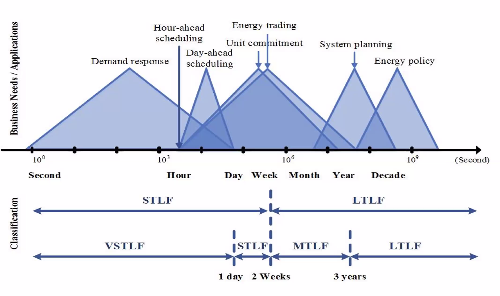
Why focus on ARIMA models

Potential

• The most widely used statistical time series forecasting approaches.

• Handle non-stationary series via differencing and seasonal patterns.

• The automatic ARIMA modeling was developed to easily implement the order selection process (Hyndman & Khandakar, 2008).

• Frequently serves asa benchmark method for forecast combinations.

Limitation

• The likelihood function of such a time series model could hardly scale up.

General framework

• The linear form makes it easy for the estimators combination

• Due to the nature of time dependence, the likelihood function of such time series model could hardly scale up, making it infeasible for massive time series forecasting.

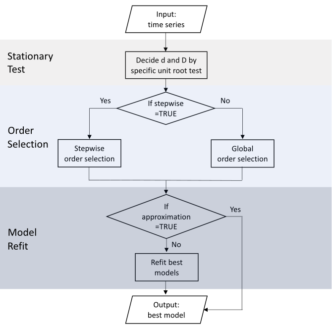
Automatic ARIMA modeling

Necessity of linear transformation

• Condition of distributed forecasting

• Local models fitted on the subseries are capable of being combined to result in the global model for the whole series.

• A seasonal ARIMA model is generally defined as \begin{align} \left(1-\sum_{i=1}^{p}\phi_{i} B^{i}\right) \left(1-\sum_{i=1}^{P}\Phi_{i} B^{im}\right)(1-B)^{d}\left(1-B^{m}\right)^{D} \left(y_{t} - \mu_0 - \mu_1 t \right) \nonumber \\ =\left(1+\sum_{i=1}^{q}\theta_{i} B^{i}\right)\left(1+\sum_{i=1}^{Q}\Theta_{i} B^{im}\right) \varepsilon_{t}. \end{align}

• Properties of ARMA models: stationarity, causality, and invertibility.

• A causal invertible model should have all the roots outside the unit circle.

• Directly combining ARIMA models would lead to a global ARIMA model with roots inside the unit circle.

• The directly combined ARIMA models will be ill-behaved, thus resulting in numerically unstable forecasts.

Linear representation

• The linear representation of the original seasonal ARIMA model can be given by \begin{equation} y_t = \beta_0 + \beta_1 t + \sum_{i=1}^{\infty}\pi_{i}y_{t-i} + \varepsilon_{t}, \end{equation} where \begin{equation} \beta_0 = \mu_0 \left( 1- \sum_{i=1}^{\infty}\pi_{i} \right) + \mu_1 \sum_{i=1}^{\infty}i\pi_{i} \qquad \text{and}\qquad \beta_1 = \mu_1 \left( 1- \sum_{i=1}^{\infty}\pi_{i} \right). \end{equation}

• This can be extended easily to involve covariates.

• For a general seasonal ARIMA model, by using multiplication and long division of polynomials, we can obtain the final converted linear representation in this form.

• In this way, all ARIMA models fitted for subseries can be converted into this linear form.

Estimators combination

• Some excellent statistical properties of the global estimator obtained by DLSA has been proved (Zhu, Li & Wang 2021, JCGS).

• We extend the DLSA method to solve time series modeling problem.

• Define $\mathcal{L}(\theta; y_t)$ to be a second order differentiable loss function, we have \begin{align} \label{eq:loss} \mathcal{L}(\theta) &=\frac{1}{T} \sum_{k=1}^{K} \sum_{t \in \mathcal{S}_{k}} \mathcal{L}\left(\theta ; y_{t}\right) \nonumber \\ &=\frac{1}{T} \sum_{k=1}^{K} \sum_{t \in \mathcal{S}_{k}}\left\{\mathcal{L}\left(\theta ; y_{t}\right)-\mathcal{L}\left(\hat{\theta}_{k} ; y_{t}\right)\right\}+c_{1} \nonumber \\ & \approx \frac{1}{T} \sum_{k=1}^{K} \sum_{t \in \mathcal{S}_{k}}\left(\theta-\widehat{\theta}_{k}\right)^{\top} \ddot{\mathcal{L}}\left(\hat{\theta}_{k} ; y_{t}\right)\left(\theta-\hat{\theta}_{k}\right)+c_{2} \nonumber \\ &\approx \sum_{k=1}^{K} \left(\theta-\hat{\theta}_{k}\right)^{\top} \left(\frac{T_k}{T} \widehat{\Sigma}_{k}^{-1}\right) \left(\theta-\hat{\theta}_{k}\right)+c_{2}. \end{align}

• The next stage entails solving the problem of combining the local

• Taylor’s theorem & the relationship between the Hessian and covariance matrix for Gaussian random variables

• This leads to a weighted least squares form

Estimators combination

• The global estimator calculated by minimizing the weighted least squares takes the following form \begin{align} \tilde{\theta} &= \left(\sum_{k=1}^{K}\frac{T_k}{T}\widehat{\Sigma}_{k}^{-1}\right)^{-1}\left(\sum_{k=1}^{K}\frac{T_k}{T}\widehat{\Sigma}_{k}^{-1}\hat{\theta}_{k}\right), \\ \tilde{\Sigma} &= \left(\sum_{k=1}^{K}\frac{T_k}{T}\widehat{\Sigma}_{k}^{-1}\right)^{-1}. \end{align}

• $\widehat{\Sigma}_{k}$ is not known and has to be estimated.

• We approximate a GLS estimator by an OLS estimator (e.g., Hyndman et al., 2011) while still obtaining consistency.

• We consider approximating $\widehat{\Sigma}_{k}$ by $\hat{\sigma}_{k}^{2}I$ for each subseries.

  • simplify the computations
  • reduce the communication costs in distributed systems.

• The global estimator and its covariance matrix can be obtained.

• The covariance matrix of subseries is not known, so we estimate it by $\sigma^2\times I$.

Output forecasts

• The $h$-step-ahead point forecast can be calculated as \begin{equation} \hat{y}_{T+h | T}=\tilde{\beta}_{0}+\tilde{\beta}_{1}(T+h)+\left\{\begin{array}{ll}\sum_{i=1}^{p} \tilde{\pi}_{i} y_{T+1-i}, & h=1 \\ \sum_{i=1}^{h-1} \tilde{\pi}_{i} \hat{y}_{T+h-i | T}+\sum_{i=h}^{p} \tilde{\pi}_{i} y_{T+h-i}, & 1<h<p. \\ \sum_{i=1}^{p} \tilde{\pi}_{i} \hat{y}_{T+h-i | T}, & h \geq p\end{array}\right. \end{equation}

• The central $(1-\alpha) \times 100 \%$ prediction interval of $h$-step ahead forecast can be defined as \begin{equation} \hat{y}_{T+h|T} \pm \Phi^{-1}\left(1-\alpha/2\right)\tilde{\sigma}_{h}. \end{equation}

• The standard error of $h$-step ahead forecast is formally expressed as \begin{equation} \tilde{\sigma}_{h}^{2} = \left\{ \begin{array}{ll} \tilde{\sigma}^{2}, & h = 1 \\ \tilde{\sigma}^{2}\left( 1 + \sum_{i=1}^{h-1}\tilde{\theta}_{i}^{2} \right), & h > 1 \\ \end{array}, \right. \end{equation} where $\tilde{\sigma}^{2}= \operatorname{tr}(\tilde{\Sigma})/p$.

Conclusions

• We propose a distributed time series forecasting framework using the industry-standard MapReduce framework.

• The local estimators trained on each subseries are combined using weighted least squares with the objective of minimizing a global loss function.

• Our framework

  • works better than competing methods for long-term forecasting.

  • achieves improved computational efficiency in optimizing the model parameters.

  • allows that the DGP of each subseries could vary.

  • can be viewed as a model combination approach.